 ### Concepts
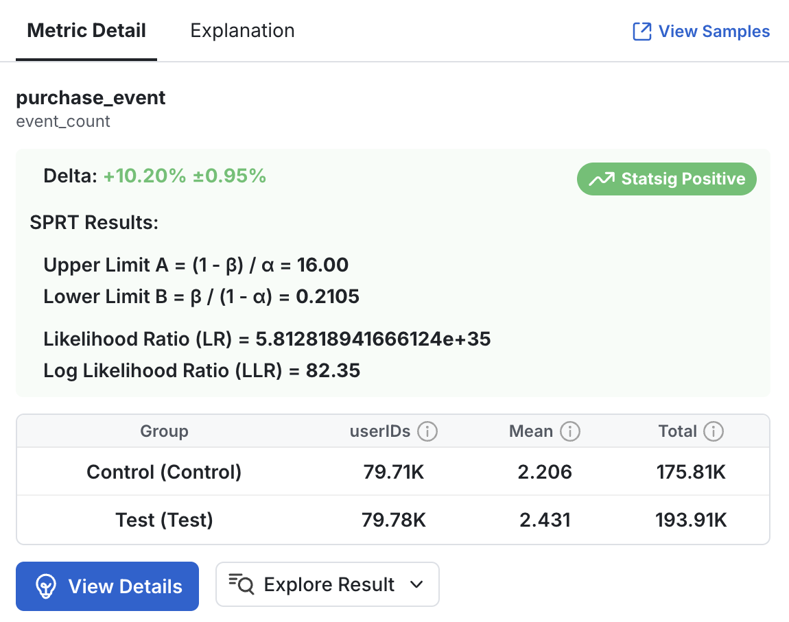
SPRT introduces a few key concepts that differ from standard Frequentist tests. At its core, SPRT relies on the **Likelihood Ratio (LR)** and Upper and Lower decision boundaries, **A** and **B**.
The Likelihood Ratio estimates the relative difference in the likelihood of two outcomes:
* **Numerator**: What you observe is due to an alternative hypothesis (you set) being correct.
* **Denominator**: What you observe is due to the null hypothesis being correct.
The Upper and Lower decision boundaries are determined by your joint tolerances for Type I and Type II errors.
* **A**: If LR exceeds this upper threshold, you should accept the Alternative Hypothesis.
* **B**: If LR is less than this lower threshold, you should accept the Null Hypothesis.
* When LR falls into the range between these thresholds, no decision can be made and you should continue collecting data.
### Concepts
SPRT introduces a few key concepts that differ from standard Frequentist tests. At its core, SPRT relies on the **Likelihood Ratio (LR)** and Upper and Lower decision boundaries, **A** and **B**.
The Likelihood Ratio estimates the relative difference in the likelihood of two outcomes:
* **Numerator**: What you observe is due to an alternative hypothesis (you set) being correct.
* **Denominator**: What you observe is due to the null hypothesis being correct.
The Upper and Lower decision boundaries are determined by your joint tolerances for Type I and Type II errors.
* **A**: If LR exceeds this upper threshold, you should accept the Alternative Hypothesis.
* **B**: If LR is less than this lower threshold, you should accept the Null Hypothesis.
* When LR falls into the range between these thresholds, no decision can be made and you should continue collecting data.
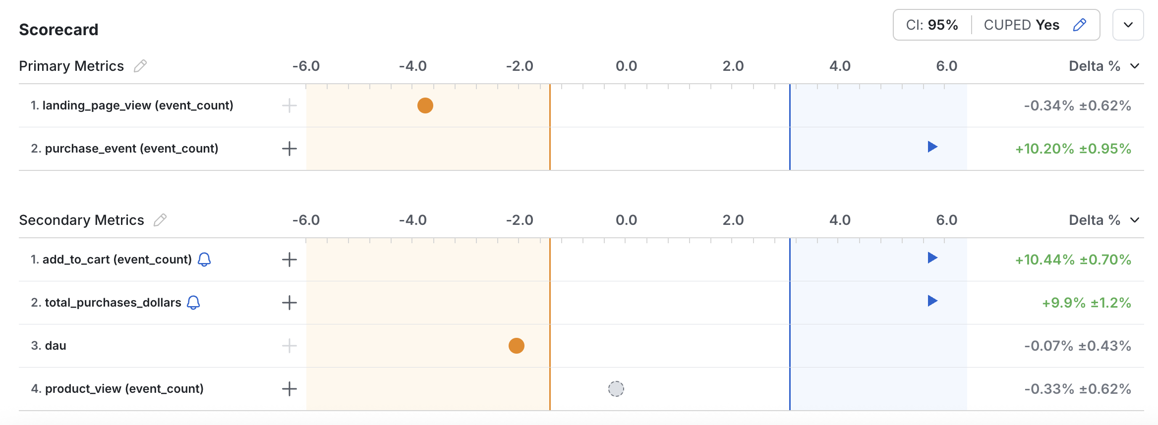
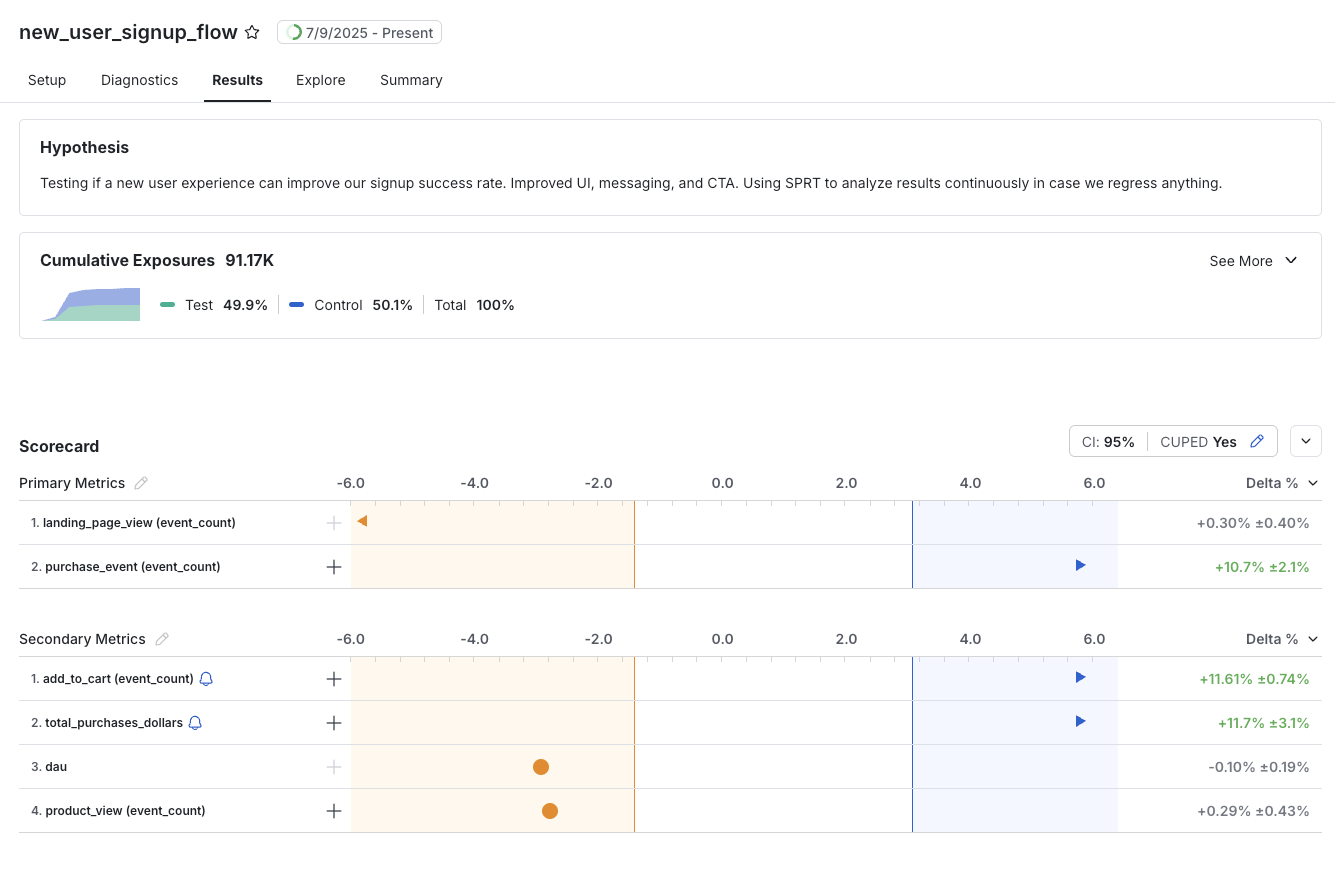
 **Interpreting Results:** The experiment Results tab shows the latest likelihood ratio for each metric in your experiment and indicates when a decision boundary has been reached, allowing you to accept the null or alternative hypothesis with confidence.
 ## Computing SPRT Results
Statsig uses an updated version of Hajnal's two-sample t test, as modified by Derek Ho of Atlassian (ref TBD), in our SPRT calculations.
On each day, compute the following for a comparison between any two groups A and B for a specific metric:
$$
{LR} =
\frac
{\phi(|z_{m}|; \theta, 1)}
{\phi(|z_{m}|; 0, 1)}
$$
where:
* $ \phi(x; \theta, 1)$ is the PDF of a normal distribution of shape $ \mathcal{N}(\theta, 1)$ evaluated at $ x$
* $ z$ is the observed Z-statistic between the groups
$$
z = \frac
{\Delta \bar{X}}
{\sigma_{\Delta\bar{X}}}
= \frac
{\bar{X}_B - \bar{X}_A}
{\sigma_{\Delta\bar{X}}}
$$
$$
\sigma_{\Delta\bar{X}}=\sqrt{\frac{var(X_A)}{N_A}+\frac{var(X_B)}{N_B}}
$$
* $ \theta$ is derived from **Cohen's d** set prior to the experiment for the particular metric being considered
$$
\theta = \frac
{\delta}
{\sqrt{
\frac{1}{N_A} + \frac{1}{N_B}
}}
$$
* $ N*{A}$ and $ N*{B}$ are the number of observed units for each group
### Power Analysis & Setting Cohen's d
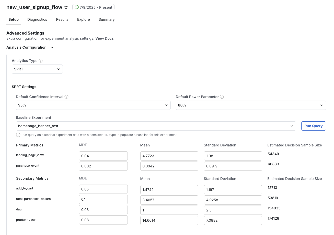
SPRT requires that a value of [**Cohen's d**](https://en.wikiversity.org/wiki/Cohen%27s_d) be set prior to the start of the experiment for each metric being evaluated. Setting the parameter requires three components:
* **MDE**: An Minimum Detectable Effect desired to be measured, in units of percent
* **Mean**: A baseline average value for the metric, $ \overline{X}$
* **Standard Deviation**: A baseline standard deviation for the metric, $ \sigma\_{X}$
With them, it's easy to compute Cohen's d parameter for each metric:
$$
\delta = \frac{\text{MDE\%} \cdot \overline{X}}{100 \cdot \sigma_{X}}
$$
This process can be automated using Statsig's built-in query tooling. If you have a past experiment that ran on a similar set of units expected in the upcoming experiment, this can be configured as a **Baseline Experiment** and a query will automatically pull the relevant metric parameters for your metrics. Users can also input all 3 parameters by hand if desired.
### Estimating the decision sample size
While Cohen's d is used to compute your experimental results after the experiment starts, it can also be used to estimate the duration of an experiment in advance. Given SPRT allows users to look at results as often as desired, this is not the same as a "required sample size" in traditional frequentist testing. The **Decision Sample Size** is an estimate of the number of samples that will be sufficient for SPRT result for a metric to exceed either threshold and accept one of the hypotheses.
Given:
$$
A=ln\left(\frac{1-\beta}{\alpha}\right)
$$
$$
k=\frac{n_{ec}}{n_{et}}=\frac{\text{units expected in control}}{\text{units expected in treatment}}=\frac{\text{\% units expected in control}}{\text{\% units expected in treatment}}
$$
$$
n_{et} = \frac{A}{\frac{1}{2}\left(\frac{k}{1+k}\right)\delta^2}
$$
Then, the total number of expected units at decision time is:
$$
n_e=n_{et}+n_{ec}=n_{et}(1+k)
$$
## References
* [Original SPRT Paper (Wald, 1945)](https://projecteuclid.org/journals/annals-of-mathematical-statistics/volume-16/issue-2/Sequential-Tests-of-Statistical-Hypotheses/10.1214/aoms/1177731118.full)
* [The Sequential Probability Ratio t Test (Schnuerch & Erdfelder, 2020)](https://martinschnuerch.com/wp-content/uploads/2020/08/Schnuerch_Erdfelder_2020.pdf)
* [A two-sample sequential t-test (Hajnal, 1961)](https://www.jstor.org/stable/2333131)
## FAQ
**Can I use SPRT for all experiments?**\
SPRT is best suited for experiments where you want faster, sequential decisions and are comfortable with likelihood-based inference. For some experiment types, traditional methods may still be preferable.
**How does SPRT affect experiment duration?**\
SPRT can reduce experiment duration, especially when there is strong evidence for or against an effect. However, if the effect is small or data is noisy, the test may run longer.
**What are the limitations?**\
SPRT requires careful setup of thresholds and assumptions. It is not a drop-in replacement for all frequentist methods, and may not be suitable for all experiment types.
**Is SPRT the same as Sequential Testing?**
SPRT is different from our Sequential Testing option. [Sequential Testing](/experiments-plus/sequential-testing) adjusts your Frequentist analysis method to allow repeated looks (i.e. "peeking"). SPRT is a completely separate experimental procedure and decision framework. They both allow for continuous "sequential" looking at experiment results, but otherwise they are separate methods for designing and running an A/B test.
## Computing SPRT Results
Statsig uses an updated version of Hajnal's two-sample t test, as modified by Derek Ho of Atlassian (ref TBD), in our SPRT calculations.
On each day, compute the following for a comparison between any two groups A and B for a specific metric:
$$
{LR} =
\frac
{\phi(|z_{m}|; \theta, 1)}
{\phi(|z_{m}|; 0, 1)}
$$
where:
* $ \phi(x; \theta, 1)$ is the PDF of a normal distribution of shape $ \mathcal{N}(\theta, 1)$ evaluated at $ x$
* $ z$ is the observed Z-statistic between the groups
$$
z = \frac
{\Delta \bar{X}}
{\sigma_{\Delta\bar{X}}}
= \frac
{\bar{X}_B - \bar{X}_A}
{\sigma_{\Delta\bar{X}}}
$$
$$
\sigma_{\Delta\bar{X}}=\sqrt{\frac{var(X_A)}{N_A}+\frac{var(X_B)}{N_B}}
$$
* $ \theta$ is derived from **Cohen's d** set prior to the experiment for the particular metric being considered
$$
\theta = \frac
{\delta}
{\sqrt{
\frac{1}{N_A} + \frac{1}{N_B}
}}
$$
* $ N*{A}$ and $ N*{B}$ are the number of observed units for each group
### Power Analysis & Setting Cohen's d
SPRT requires that a value of [**Cohen's d**](https://en.wikiversity.org/wiki/Cohen%27s_d) be set prior to the start of the experiment for each metric being evaluated. Setting the parameter requires three components:
* **MDE**: An Minimum Detectable Effect desired to be measured, in units of percent
* **Mean**: A baseline average value for the metric, $ \overline{X}$
* **Standard Deviation**: A baseline standard deviation for the metric, $ \sigma\_{X}$
With them, it's easy to compute Cohen's d parameter for each metric:
$$
\delta = \frac{\text{MDE\%} \cdot \overline{X}}{100 \cdot \sigma_{X}}
$$
This process can be automated using Statsig's built-in query tooling. If you have a past experiment that ran on a similar set of units expected in the upcoming experiment, this can be configured as a **Baseline Experiment** and a query will automatically pull the relevant metric parameters for your metrics. Users can also input all 3 parameters by hand if desired.
### Estimating the decision sample size
While Cohen's d is used to compute your experimental results after the experiment starts, it can also be used to estimate the duration of an experiment in advance. Given SPRT allows users to look at results as often as desired, this is not the same as a "required sample size" in traditional frequentist testing. The **Decision Sample Size** is an estimate of the number of samples that will be sufficient for SPRT result for a metric to exceed either threshold and accept one of the hypotheses.
Given:
$$
A=ln\left(\frac{1-\beta}{\alpha}\right)
$$
$$
k=\frac{n_{ec}}{n_{et}}=\frac{\text{units expected in control}}{\text{units expected in treatment}}=\frac{\text{\% units expected in control}}{\text{\% units expected in treatment}}
$$
$$
n_{et} = \frac{A}{\frac{1}{2}\left(\frac{k}{1+k}\right)\delta^2}
$$
Then, the total number of expected units at decision time is:
$$
n_e=n_{et}+n_{ec}=n_{et}(1+k)
$$
## References
* [Original SPRT Paper (Wald, 1945)](https://projecteuclid.org/journals/annals-of-mathematical-statistics/volume-16/issue-2/Sequential-Tests-of-Statistical-Hypotheses/10.1214/aoms/1177731118.full)
* [The Sequential Probability Ratio t Test (Schnuerch & Erdfelder, 2020)](https://martinschnuerch.com/wp-content/uploads/2020/08/Schnuerch_Erdfelder_2020.pdf)
* [A two-sample sequential t-test (Hajnal, 1961)](https://www.jstor.org/stable/2333131)
## FAQ
**Can I use SPRT for all experiments?**\
SPRT is best suited for experiments where you want faster, sequential decisions and are comfortable with likelihood-based inference. For some experiment types, traditional methods may still be preferable.
**How does SPRT affect experiment duration?**\
SPRT can reduce experiment duration, especially when there is strong evidence for or against an effect. However, if the effect is small or data is noisy, the test may run longer.
**What are the limitations?**\
SPRT requires careful setup of thresholds and assumptions. It is not a drop-in replacement for all frequentist methods, and may not be suitable for all experiment types.
**Is SPRT the same as Sequential Testing?**
SPRT is different from our Sequential Testing option. [Sequential Testing](/experiments-plus/sequential-testing) adjusts your Frequentist analysis method to allow repeated looks (i.e. "peeking"). SPRT is a completely separate experimental procedure and decision framework. They both allow for continuous "sequential" looking at experiment results, but otherwise they are separate methods for designing and running an A/B test.